Using MCMC to manipulate images

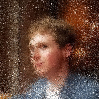
A few years ago, I was interested in exploring some ideas around the content of images and vision, and in trying to think of ways of reconstructing images from smaller amounts of information. At this point those who are “technically inclined” may think of compression techniques or using wavelet bases, but I was interested in doing something a bit more artistic. In playing around with this, I ended up coming up with an idea based around sampling a small percentage of pixels in the image and drawing paths between them, which to me gives rise to some interesting looking images:

As it wouldn’t take me too long to share, I’ve written up a short post explaining what is going on, along with sharing code to allow you to play around with it. While I have the code in a GitHub repo, downloading and installing Python packages takes some time, so I also have a Google Colab notebook which will allow you to more easily have five minutes of playing around and having some fun with it. If you’re interested in how it works, I have an explaination below; otherwise, I hope it gives you some fun moments of distraction!

What’s happening under the hood?

The procedure to generate these images has a few different steps, with the underlying idea being to use MCMC methods (in this case, a Metropolis-Hastings algorithm with a Gaussian proposal distribution) in order to sample pixels from the image, and then use this as a basis for “reconstructing” the image.

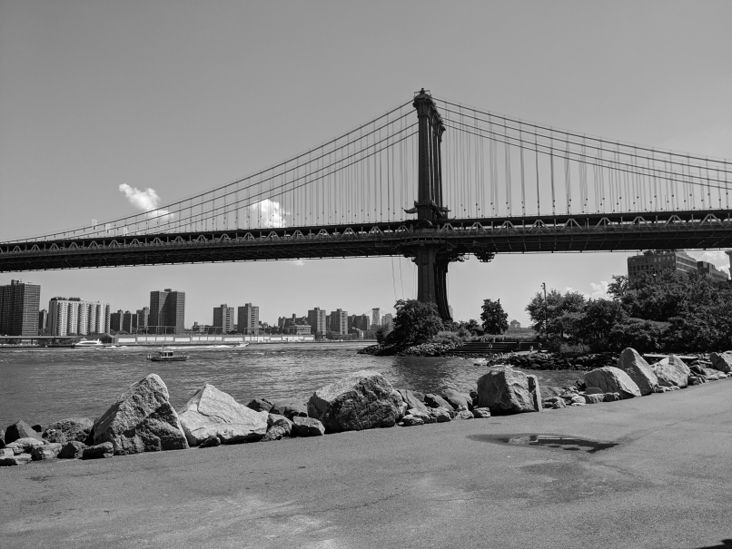
To do this, we first need a generate an underlying density over the pixels of the image to use as our target distribution for the MCMC sampler. After some experimenting, what I found to give the “best looking” results was to use the “lightness” channel of an image to use as the density, so that light areas of the image had low density (with pure white areas having no density), and darker areas of the image having higher density.

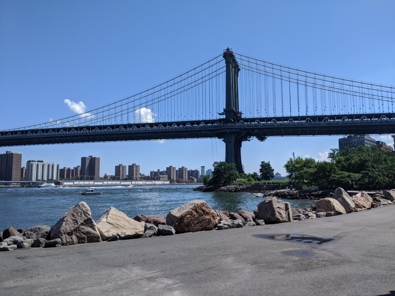
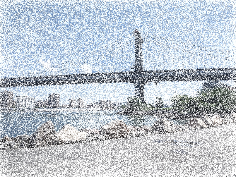
For example, if we start with this image from this picture of the Manhattan Bridge:

then after extracting the luminosity channel we are left with:

To go into a bit more detail as to how the density is created, it is important to be aware that computer images are thought of as being blends of Red, Green and Blue, with each of these colours being referred to as channels. For every pixel in our image, we have a vector of three integers (corresponding to each channel) between 0 and 255.

If you’re familiar with the idea of coordinate changes, then you can imagine that we could transform our channels to be in a different coordinate system. One way of doing so is to map the channels to the CIELAB or L*a*b* color space, in which case the first channel corresponds to the “lightness” or luminosity of the pixel, and is designed to roughly correspond to what we would perceive as “how much light” a particular area (or in this case, a pixel), would have. After negating this channel, we then end up with the density for proposing pixels.

Let’s call this density $p(x)$, where $x \in I$ corresponds to a pixel in our image $I$. To then create a sample of points $x_0, \ldots, x_M$, if we have a pixel $x_i$, we’ll first sample a proposed pixel $y_i$ from the distribution

where the indicator term is used to ensure that our proposed pixel remains within the image, and $h$ is a given bandwidth which controls how far $y_i$ can be from $x_i$. (Here, we’ll ignore the fact that this is a continuous distribution and pixels are discrete; in practice, we just round the coordinates generated to the nearest integer.)

Once we have this, we compute the value

and then let $x_{i+1} = y_i$ with probability equal to the value computed above, and otherwise let $x_{i+1} = x_i$. Repeating this process then gives us a sequence of pixels.

On its own, we could just use the sampled pixels to reconstruct the image by only rendering the image at these points. However, this doesn’t give very interesting images - either there is too little going on, or we need to sample most of the pixels to see anything.

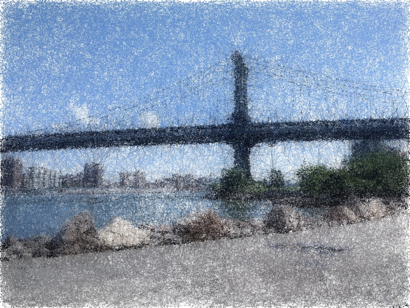
What I found to be more interesting was to draw lines between concurrent pixels, and using the same color at the starting location for the line until arriving at the next pixel. This then gives rise to images where you can identify what is in the image, but in a far more visually compelling way to before, while still only needing the same amount of information.

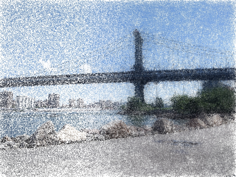
By rendering images these way, I only need to usually sample five to ten percent of the pixels of the image to retain some perspective of the individual image. (For reference, saving an image as a .jpg will achieve a similar level of compression - although clearly for day to day purposes, you should use that.)